Bin-by-bin Likelihood Profiles
This page describes formats for bin-by-bin likelihood profiles as currently used in some LAT analyses. The bin-by-bin likelihood extends the concept of an SED by providing a representation of the likelihood function in each energy bin. Likelihood SED and Likelihood SED Cube are two formats for serializing bin-by-bin likelihoods to a FITS file. A Likelihood SED stores the bin-by-bin likelihood for a single source or test source position while a Likelihood SED Cube stores a sequence of bin-by-bin likelihoods (e.g. for a grid of positions or a group of sources).
In the following we describe some advantages and limitations of using bin-by-bin likelihoods. Relative to a traditonal SED, the bin-by-bin likelihood retains more information about the shape of the likelihood function around the maximum. This can be important when working in the low statistics regime where the likelihoods are non-Gaussian and a flux value and one sigma uncertainty is insufficient to describe the shape of the likelihood function. Applications in which bin-by-bin likelihoods may be useful include:
- Deriving upper limits on the global spectral distribution of a source. Likelihood SEDs can be used to construct the likelihood function for arbitrary spectral models without recomputing the experimental likelihood function. This is particularly useful for DM searches in which one tests a large number of spectral models (e.g. for mass and annihilation channel) and recomputing the experimental likelihood function for all models would be very expensive. The bin-by-bin likelihoods are also a convenient way of distributing analysis results in a format that allows other spectral models to be easily tested. The two of the most recent LAT publications on dSph DM searches have publicly released the analysis results in this format (see 2015PhRvL.115w1301A and 2014PhRvD..89d2001A).
- Stacking analyses that combine measurements from multiple sources or multiple epochs of observation of a single source. Forming a joint likelihood from the product of Likelihood SEDs fully preserves information in each data set and is equivalent to doing a joint fit as long as the data sets are independent.
- Analyses combining spectral measurements from multiple experiments. Likelihoods from two or more experiments can be multiplied to derive a joint likelihood function incorporating the measurements of each experiment. As for stacking analyses, the joint likelihood approach avoids merging or averaging data or IRFs. The bin-by-bin likelihoods further allow joint anlayses to be performed without having access to the data sets or tools that produced the original measurement. For an application of this approach in the context of DM searches see 2016JCAP…02..039M.
There are a few important caveats to bin-by-bin likelihoods which may limit their use for certain applications:
- Large correlations between the normalizations of two or more model components (e.g. when the spatial models are partially degenerate) can limit the utility of this approach. Although such correlations can be accounted for by profiling the corresponding nuisance parameters, this may result in unphysical background models with large bin-to-bin fluctuations in the model amplitude. One technique to avoid this issue (see 2015PhRvD..91j2001B and 2016PhRvD..93f2004C) is to apply a Gaussian prior that constrains the spectral distribution of the background components to lie within a certain range of the global spectral model of that source (computed without the test source).
- Because the likelihoods in each energy bin are calculated independently, this technique cannot fully account for bin-to-bin correlations caused by energy dispersion. The effect of energy dispersion can be corrected to first order by scanning the likelihood with a spectral model (e.g. a power-law with index 2) that is close in shape to the spectral models of interest. However in analyses where the energy response matrix is particularly broad or non-diagonal the systematic errors arising from the approximate treatment of energy dispersion may exceed the statistical errors. In LAT analyses energy dispersion can become a significant effect when using data below 100 MeV (see LAT_edisp_usage). However when using an Index=2.0 and considering energies above 100 MeV, the spectral bias is less than 3% for models with indices between 1 and 3.5.
Likelihood SED
The likelihood SED is a representation of spectral energy distribution of a source that contains a likelihood for the source normalization in each energy bin. This format is a special case of the more general SED format. Depending on the requirements of the analysis the likelihoods can be evaluated with either profiled or fixed nuisance parameters. The likelihood SED can be used in the same way as a traditional SED but contains additional information about the shape of the likelihood function around the maximum. A 2D visualization of the likelihood functions can be produced by creating a colormap with intensity mapped to the likelihood value:
| Low Significance Source | High Significance Source |
|---|---|
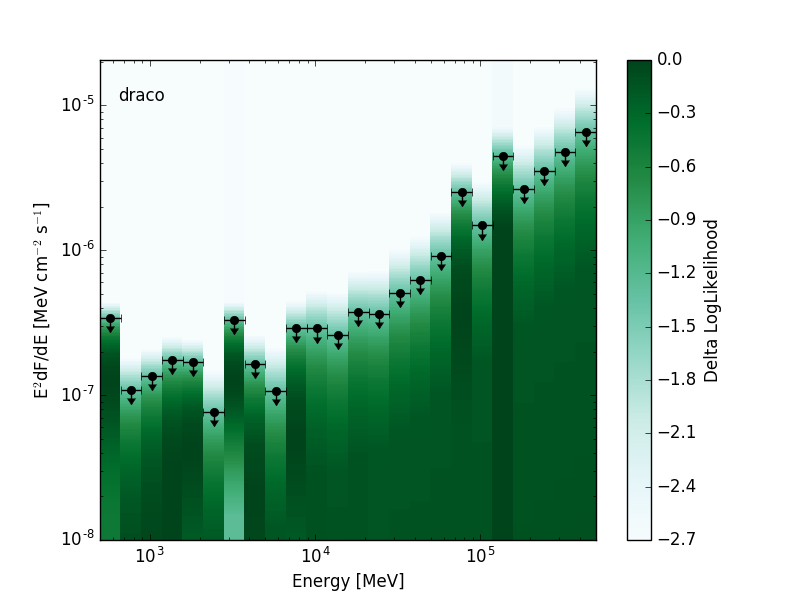 |
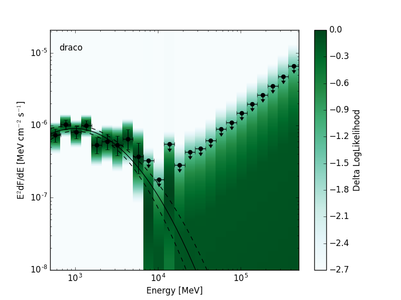 |
In the following we use nebins to designate the number of energy bins and nnorms to designate the number of points in the normalization scan. The format is a BINTABLE with one row per energy bin containing the columns listed below.
The best-fit model amplitudes, errors, and upper limits are all
normalized to a reference spectral model. The ref columns define
the amplitude of the reference model in different units. The
reference model amplitudes are arbitrary and could for instance be set
to the best-fit amplitude in each energy bin. norm columns
contain the best-fit value, its errors, and upper limit in units of
the reference model amplitude. Unit conversion of the norm
columns can be performed by doing a row-wise multiplication with the
respective ref column.
Sample Files
See the likelihood files in Sample Files.
Header Keywords
SED_TYPE- SED type string. Should be set to
likelihood.
- SED type string. Should be set to
UL_CONF, optional- Confidence level of the upper limit (range: 0 to 1) of the value in the
norm_ulcolumn.
- Confidence level of the upper limit (range: 0 to 1) of the value in the
Columns
The columns listed here are a subset of the columns defined in the SED format. See Columns for the full column specifications.
Required Columns
e_min– ndim: 1, Dimension: nebinse_max– ndim: 1, Dimension: nebinse_ref– ndim: 1, Dimension: nebinsref_dnde– ndim: 1, Dimension: nebinsref_eflux– ndim: 1, Dimension: nebinsref_flux– ndim: 1, Dimension: nebinsref_npred– ndim: 1, Dimension: nebinsnorm– ndim: 1, Dimension: nebinsnorm_err– ndim: 1, Dimension: nebinsnorm_scan– ndim: 2, Dimension: nebins x nnormsts– ndim: 1, Dimension: nebinsloglike– ndim: 1, Dimension: nebinsdloglike_scan– ndim: 2, Dimension: nebins x nnorms
Optional Columns
ref_dnde_e_min– ndim: 1, Dimension: nebinsref_dnde_e_max– ndim: 1, Dimension: nebinsnorm_errp– ndim: 1, Dimension: nebinsnorm_errn– ndim: 1, Dimension: nebinsnorm_ul– ndim: 1, Dimension: nebins
Likelihood SED Cube
The Likelihood SED Cube is format for storing a sequence of Likelihood SEDs in a single table. The format defines a file with two BINTABLE HDUs: SCANDATA and EBOUNDS. SCANDATA has one row per Likelihood SED while EBOUNDS has one row per energy bin. Table rows in SCANDATA can be mapped to a list of sources, spatial pixels, or observations epochs. Because the row mapping is not defined by the format itself additional columns can be added to SCANDATA that defined the mapping of each row. Examples would be columns for source name designation, pixel coordinate, or observation epoch.
In the following we use nrows to designate table rows, nebins to
designate the number of energy bins and nnorms to designate the
number of points in the normalization scan. As for the Likelihood SED
format, columns that contain norm are expressed in units of the
reference model amplitude. These can be multiplied by ref_eflux,
ref_flux, ref_dnde, or ref_npred columns in the EBOUNDS
HDU to get the normalization in the respective units.
Sample FITS files:
- Low Significance Source:
tscube_lowts.fits - High Significance Source:
tscube_hights.fits
SCANDATA Table
The SCANDATA HDU is a BINTABLE with the following columns. The columns listed here are a subset of the columns in the SED format. Relative to the 1D SED formats the dimensionality of all columns is increased by one with the first dimension (rows) mapping to spatial pixels. See Columns for the full column specifications.
Header Keywords
UL_CONF, optional- Confidence level of the upper limit given in the
norm_ulcolumn.
- Confidence level of the upper limit given in the
Required Columns
dloglike_scan– ndim: 3, Dimension: nrows x nebins x nnormsnorm_scan– ndim: 3, Dimension: nrows x nebins x nnormsnorm– ndim: 2, Dimension: nrows x nebinsnorm_err– ndim: 2, Dimension: nrows x nebinsts– ndim: 2, Dimension: nrows x nebinsloglike– ndim: 2, Dimension: nrows x nebins
Optional Columns
ref_npred– ndim: 2, Dimension: nrows x nebinsnorm_errp– ndim: 2, Dimension: nrows x nebinsnorm_errn– ndim: 2, Dimension: nrows x nebinsnorm_ul– ndim: 2, Dimension: nrows x nebinsbin_status– ndim: 2, unit: None- Dimension: nrows x nebins
- Fit status code. 0 = OK, >0 = Not OK
EBOUNDS Table
The EBOUNDS HDU is a BINTABLE with 1 row per energy bin and the following columns. The columns listed here are a subset of the columns in the SED format. See Columns for the full column specifications. Note that for backwards compatibility with existing EBOUNDS table convention (e.g. as used for WCS counts cubes) columns names are upper case.
Required Columns
E_MIN, unit: keV, Dimension: nebinsE_REF, unit: keV, Dimension: nebinsE_MAX, unit: keV, Dimension: nebinsREF_DNDE– ndim: 1, Dimension: nebinsREF_EFLUX– ndim: 1, Dimension: nebinsREF_FLUX– ndim: 1, Dimension: nebins
Optional Columns
REF_DNDE_E_MIN– ndim: 1, Dimension: nebinsREF_DNDE_E_MAX– ndim: 1, Dimension: nebinsREF_NPRED– ndim: 1, Dimension: nebins
TSCube Output Format
Recent releases of the Fermi ScienceTools provide a gttscube application that fits a test source on a grid of spatial positions within the ROI. At each test source position this tool calculates the following information:
- TS and best-fit amplitude of the test source.
- A likelihood SED.
The output of the tool is a FITS file containing a Likelihood SED Cube with nrows in which each table row maps to a pixel in the grid scan. The PRIMARY HDU contains the same output as gttsmap – a 2-dimensional FITS IMAGE with the test source TS evaluated at each position. The primary fit results are contained in the following BINTABLE HDUs:
- A SCANDATA Table containing the likelihood SEDs for each spatial pixel.
- A FITDATA Table containing fit results for the reference model at each spatial pixel over the full energy range.
- A EBOUNDS Table containing the bin definitions and the amplitude of the reference model.
The mapping of rows to pixels is defined by the WCS header keywords in the SCANDATA HDU. Following the usual FITS convention both tables use columnwise ordering for mapping rows to pixel indices.
Here is the list of HDUs:
| HDU | HDU Type | HDU Name | Description |
|---|---|---|---|
| 0 | IMAGE | PRIMARY | TS map of the region using the test source |
| 1 | BINTABLE | SCANDATA | Table with the data from the likelihood v. normalization scans. Follows format specification given in SCANDATA Table. |
| 2 | BINTABLE | FITDATA | Table with the data from the reference model fits. |
| 3 | BINTABLE | BASELINE | Parameters and Covariences of Baseline fit. |
| 4 | BINTABLE | EBOUNDS | Energy bin edges, fluxes and NPREDs for test source in each energy bin. Follows format specification given in EBOUNDS Table. |
FITDATA Table
The FITDATA HDU is a BINTABLE with 1 row per spatial pixel (nrows) and the following columns:
fit_norm– ndim: 1, unit: None- Dimension: nrows
- Best-fit normalization for the global model in units of the reference model amplitude.
fit_norm_err– ndim: 1, unit: None- Dimension: nrows
- Symmetric error on the global model normalization in units of the reference model amplitude.
fit_norm_errp– ndim: 1, unit: None- Dimension: nrows
- Positive error on the global model normalization in units of the reference model amplitude.
fit_norm_errn– ndim: 1, unit: None- Dimension: nrows
- Negative error on the global model normalization in units of the reference model amplitude.
fit_norm_ul– ndim: 1, unit: None- Dimension: nrows
- Upper limit on the global model normalization in units of the reference model amplitude.
fit_ts– ndim: 1, unit: None- Dimension: nrows
- Test statistic of the best-fit global model.
fit_status– ndim: 1, unit: None- Dimension: nrows
- Status code for the fit. 0 = OK, >0 = Not OK